home

contents Mathematics

previous :    birth of a dimension

next :    chains of dimensions

To see what's going on in the 4^th dimension

How many simultaneous dimensions can we represent and read in a continuous way? Three for the three dimensions of space, and one fore time dimension, then it makes four.
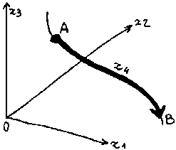
To get these 4 dimensions we make a frame of 3 dimensions of coordinates, and in this frame we represent the location of a moving body at various times. It's a usual 3 D + T diagram: in it we 'hold back' the successive locations of the body in its move, the ones besides the others, which enables us to represent the 4th dimension, time dimension.
 

evolution of the body from A to B in 4 simultaneous dimensions It's the continuous line AB that represents the continuity of the 4th dimension, generally use to represent time dimension

So, in this 'usual use', the continuity between different points of a 3 D space is used to represent the continuity of what happens in time dimension, but we can also use it to represent the continuity of another dimension than time dimension. In fact, the continuity of any type of dimension of value 1.

We can therefore consider using such a diagram with 3 D + 1 dimensions to represent the 4 dimensions of a 4 D + T deformation, provided we give up the idea of representing simultaneously its time dimension.
In the case of a phenomenon that gains a 4th self-similarity dimension, that's what is happening in a continuous way in this dimension of self-similarity that can be represented instead of what is happening in a continuous way in time dimension.

Now, we understand that it's very precisely this, that the Robert Shaw's team got in the diagram which 'faked' the 1 D series of the chaotic phase of the dripping tap [to see again    this diagram].
Every dimension of the 3 D diagram (abscissa, ordinate, height) holds the values of all measured time intervals, but as these values are shifted of one step between each dimension, the continuity that appears on the 4th dimension of the graph is what is 'transverse' of all the measured time intervals. And what is transverse to time dimension where they were produced, and what is also transverse to every deformation that produced them, that's precisely the interference of the deformations, which happens to be, in this phase of the phenomenon, self-similar.
Then, what the graph shows, is the look of the continuous deformation of self-similarity provoked by the interference of the 3 initial deformations of the phenomenon.
As there is only room on this diagram for 4 continuous deformations, the self-similarity deformation replaces time dimension there. We have explicitly given up time dimension when gathering time intervals in triples, for in these triples every time interval is not only confronted with the time interval that follows it in time, but also with that which follows the following: we then jump over the strict continuity of what follows in time, we broke the 1 D ordering of time. As a result, on this 4 D diagram (4 deformations), a point and its following in time have no relation of continuity, therefore no relation of proximity.
 

Now we are coming to the very look of a diagram which represents a dimension of self- similarity.
When the 4th dimension of a 3 D + 1 D diagram represents the continuity of time dimension, its aspect is a continuous curve: every successive point of this curve touches one another, exactly as every successive sequence of time touches one another.
Then, when the 4th dimension represents the dimension of self-similarity we must expect it to look like a self-similar diagram, for in the same way as a continuous movement has a continuous curve as 'image', a self-similar dimension has to have a self-similar diagram as 'image'.
And this is precisely what we got.
We cannot observe it in the case of the attractor drawn by the Shaw team, for it's a 'blurred' diagram, but we know that this diagram is a partial cross-section of an attractor known as 'Rössler's attractor'.
 
 

Rössler attractor the diagram obtained by Shaw team is a partial cross-section of this attractor [to see again   this diagram] [this drawing is from James P. Crutchfield in an article 'le Chaos' in 'Pour la Science']

It happens that mathematicians call the Rössler attractor a 'strange' attractor for it repeats itself in every of its scales, that is, every time we look at it on a tinier scale we got the same pattern as the pattern we got in the big ones.
We shall observe this special feature on another 'strange attractor', which is called the Hénon attractor, from Michel Hénon who invented it.

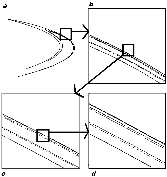
self-similarity of Hénon attractor in all its scales [the drawings are from P. Crutchfield]   This curve is mathematically calculated, and with the help of simulation calculation we can examine it as under a microscope which enlarges 1000 times.  Thus, the diagram show in a an overall view of the curve which represents the successive positions of the same start point. In b, is a 10 times enlargement of the small square of a. In c, is a 10 times enlargement of the small square of b. And finally in d, is a 10 times enlargement of the small square of c. Then in d is a 1000 times enlargement of a detail of a, which looks like the overall pattern of the central part of a. In the same time, d represents a part of c banding which is so much similar to c and b banding in their number and in their rhythm of succession (2 very closed lines on the outer side, then a small gap, then 2 relatively closed lines, then a medium gap, then 2 extremely closed lines on the inner side), that it is impossible to differentiate a view and a 10 times smaller view or a 100 times smaller view, except for the radius of the curve which slowly change from one diagram to another. It's hard to believe that the 4 double-lines in the 'd' diagram are nothing but the enlargement of the 2 external double-lines in the 'c' diagram, and when we understand this, we expect that, provided the calculation unables us to enlarge 10 times more the diagram, we should see the same pattern in 4 double-lines in the enlargement of the external lines of d. Whatever the scale, the detail in the detail is absolutely the same as the detail in the detail in the detail, etc. [note: simulations of Hénon attractor show the same self-similar structure in the sharp part of the diagram a as in the central part of a, and with the same pattern of banding. Then, these two parts are only differenciated by the radius of the curve, which is modered in the central part, and very sharp in the other] The shape in one aspect of this figure. There is another aspect we cannot see when the diagram is over, but when we look at the successive positions of the points as the calculation is under process: the point does not move in a regular and seemingly logic way, but moves with an irregular rhythm which is impossible to predict. For instance it will be lingering a long time in a corner of the diagram, then it will suddenly escape in a far away corner that it will quickly leave, or where it will stay a long time, always like by chance. We have already explained the cause of this chaotic movement of the point: the dimension of time continuity has vanished to make room for the dimension of self-similarity dimension, for the diagram does not have enough dimensions to simultaneously represent these two dimensions.

So, strange attractors spread on surfaces with variable density, not on lines.
This is the remaining mystery, for this is not directly obvious.
In the same way as the continuity of a movement in time dimension is represented by a continuous curve, we could have expected that the continuity of self-similarity dimension would be represented by a continuous self-similar curve.
For self-similar curves do exist: we have seen such a curve already.
For instance, strange attractor could be something like the von Kock's snowflake curve [to see it     again], rather than being something like the Peano's curve/surface [to see it     again].
 

We have understood the reason why a point makes random jumps in time dimension,
but why does it make its jumps on a surface rather than on a line?
 
 
 
 

home

Math

top

next :      chains of dimensions

author